Notes for: PostgreSQL Query Optimization: The ultimate guide to building efficient queries

47 minute read

title: PostgreSQL Query Optimization: The ultimate guide to building efficient queries author: Dombrovskaya H., Novikov B. and Bailliekova A. published: 2021 edition: 1 ISBN: 978-1484268841

Why Optimise

Optimisation starts with gathering requirements about the use case the system is serving.
- normalise or denormalise tables, to serve use cases that might require searching a smaller set of data.
- unique and primary identifier concerns.
- frequency of access.
- acceptable response time (mission critical apps vs report generation has different tolerance).
- resource consumption
- throughput required
- think about optimised query as early as possible in the application development
- questioning the business intent of queries, may help us find elegant solutions that avoid complex queries all together.
Two key concepts to think like a database:
- how a database engine processes a query
- how a query planner decides what execution path to choose
Even though SQL is declarative, we may construct queries in imperative fashion and end up having hard-coded execution path, which can never be optimised by the database engine.

--imperative
SELECT *
FROM student
WHERE class_id in
      (SELECT class_id FROM class WHERE cohort_year = '2021');

-- declarative
SELECT *
FROM student st
         join class cl ON st.class_id = cl.id
WHERE cl.cohort_year = '2021';

Two main classes of systems:
- OLTP (Online Transaction Processing) systems, usually optimised for short queries.
- OLAP (Online Analytical Processing) systems, usually optimised for both long and short queries.
Observe performance trends.
- Query may degrade over time as volume of data increase or distribution of data changes.
- We may also need to update queries for new PostgreSQL release and features.

PostgreSQL quirks

PostgreSQL has different implementation compared to other databases.
Optimisation techniques specific to other databases may not be applicable to PostgreSQL.
It is important to be aware of new features and releases and consider how they can be used for our apps.
For example, PostgreSQL by design does not accept hints from users.
- The query planner will choose the best path independently.
- Users simply focus on writing declarative SQL queries.

Processing and Operations

Processing Overview

1. Compilation
- Different DB servers can interpret the same SQL query differently.
- Compiled SQL queries are declarative high-level logical operations (logical plan), which does not determine final execution.
2. Optimization
- Optimiser replaces logical operations with their execution algorithms by choosing the best out of possible algorithms.
- Optimiser may change the logical expression structure by changing the order in which logical operations will be executed.
- Optimiser seeks to minimise physical resources used (including execution time) by choosing the best physical operations (execution plan) for the given logical plan.
3. Execution
- The executor simply runs the plan and return the results.

Relational Operations

Theoretical.
We can simplify relational theory by assuming a relation is a table.
Any relational operations take one of more relations as input, and produces another relation as output. Relational operations can therefore be chained.
filter: returns all rows from the input relation that satisfy filter condition.
project: returns the input relation with some attributes removed and rows de-duplicated.
product: (a.k.a. Cartesian product) returns all pairs of rows from two input relations.
The SQL JOIN is simply a product followed by a filter operation.
Other operations include grouping, union, intersection, and set difference
All operations satisfy the equivalence rules:
- Commutativity: JOIN(R,S) = JOIN (S,R)
- Associativity: JOIN(R, JOIN(S,T)) = JOIN(JOIN(R,S), T)
- Distributivity: JOIN(R, UNION(S,T)) = UNION(JOIN(R,S), JOIN(R, T))

Logical Operations

Logical operations extends the capabilities of relational operations to support SQL constructs.
Operations also obeys equivalence rules. Equivalence rules is the key to allowing the optimiser to use different expressions to produce the same output.
Chaining those operations works like pure functions (no side effects), which is optimal for database query performance.
It is easier for humans to think about operations working on a set (or a table) than to think about iterating over individual rows of data, to write better declarative queries.

Algorithms

Logical operations are implemented as algorithms (sometimes with a few alternative implementation per operation)
Query planner will choose the best algorithm to use to optimise resource consumption.
Multiple algorithms may need to work in sequence (data access, followed by transformation) to support a single logical operation.

Algorithm Cost Models

The primary metrics are CPU cycles and I/O accesses.
Available memory, memory distribution, also affects the ratio of primary metrics (but this is server params, out-of-scope).
Query optimiser uses a single composite of both metric to compare cost across different algorithms.
The cost metric used to be dominated by I/O accesses (because hard drives rotation are more expensive) but for modern hardware (e.g. SSD) this may not be relevant.
Optimiser should be tuned to consider modern hardware (again, this is server params, out-of-scope).
Cost also depends on input table to the operation.
- R = table
- TR = number of rows
- BR = number of storage blocks occupied by table

Data Access Algorithms

These operations are usually combined with subsequent operations. E.g. filtering rows after reading from table is less efficient than simply reading the required rows.
Selectivity: Ratio between total number of rows in table vs rows that will be retained after the operations
Choice of read algorithm is influenced by selectivity of subsequent filter operations, that can be simultaneously applied.

Storage Structures

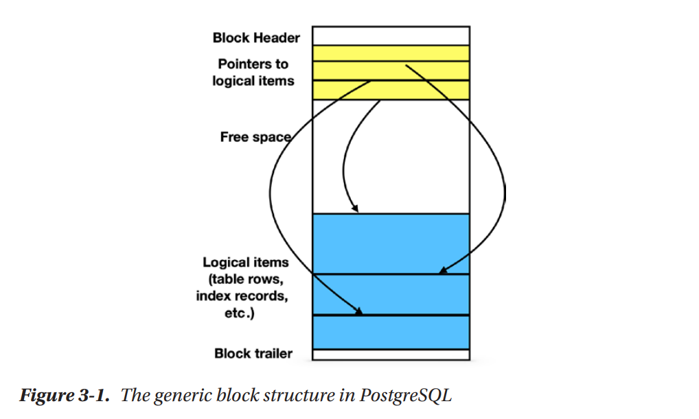
Data are stored as files in hard drives.
Files used for database objects (rows, tables, indexes …) are divided in blocks of the same length (PostgreSQL by default uses 8192 bytes or 8Kb per block)
Several small items may reside in a single block, large items may span multiple blocks.
The allocation of items to blocks also depends on the type of the database object (e.g. a table uses the heap data structure).
A block is the unit transferred between hard drive and main memory.
Therefore, the number of I/O operations = number of blocks transferred during a read/write.

![[image-postgresql-harddisk-block.png]]

Full Scan

Cost of full scans with a filter condition is simply

cost of total blocks read from the table +
cost of total rows processed in memory +
cost of filter (determined by selectivity, annotated as S) multiplied by total number of rows

cost = (c1 * BR) + (c2 * TR) + (c3 * S * TR)

where cX are hardware dependent constants.

Index-Based Table Access

Tables store rows in heap data structure, therefore rows are unordered.
Indexes provide additional data access path, for us to determine where data is stored without scanning the table.
Two physical operations to read retrieve rows via indexes:
First, the index scan:
- the algorithm scans index for pointers to all rows that satisfy condition.
- the entire block that contains the row will be read.
- as the table uses heap, multiple rows may be stored on the same block.
- the same block may be retrieved multiple times (inefficient)
Second, the bitmap heap scan:
- a bitmap indicating blocks that contain needed rows are first generated.
- then all the rows in those blocks are filtered for those we need.
- very efficient to generate multiple bitmaps from multiple indexes, then use them all in a single query (bitmaps can be evaluated together using logical AND/OR)
The cost of such access is approximately:
- for low selectivity, rows are sparsely distributed, fewer blocks will be retrieved, so cost is proportional to number of rows retrieved.
- for high selectivity, almost all blocks will be retrieved (perform worse than full scan due to additional steps to read indexes and generate bitmaps)

Index-Only Scan

Index-only scan takes place when we combine project operation with data access, and all the columns needed in the projection are also in the index.
The cost of such access is approximately:
- proportional to number of rows retrieved (for all levels of selectivity)
- for high selectivity, it will still perform better than the above access types, because retrieval contains less data.

Comparing Data Access Algorithms

In general:

index-only scan has the best performance and is preferred.
index-based table access is better than full scan for low selectivity.
full scan execution cost is almost constant, regardless of selectivity, and will be better than index-based table access for high selectivity use cases.

Choosing the best algorithm then depends on use cases.

Any algorithm can become a winner under certain conditions.
Decision also depends on storage structures and statistical properties of the data. The database maintains metadata (statistics) for tables, e.g. column cardinality, sparseness. Such statistics change over the lifecycle of the app.
The declarative nature of SQL is essential, to allow query optimiser to use all the above information to select the best execution plan for the same SQL query.

Index Structures

Instead of using structural properties, we will define an index based on its usage. It must be:

a redundant data structure (in relation to the table).
transparent to user/apps.
designed to improve query performance.

Index update when rows are updated introduces some overhead, but modern RDBMS has algorithm to optimise such updates.

Unlike other databases, PostgreSQL does not have clustered indexes. All tables are heap tables, all indexes are non-clustered. (Clustered index defines the order in which data is physically stored in a table)

B-Tree Indexes

(Using a student table as example, with PK student_id we want to index by name)

B-Tree is also known as self-balancing tree. Nodes can have more than 2 children.
Nodes are associated with blocks on the disk.
Leaf nodes contain actual index records (the indexed key, maps to table row id e.g. name maps to student_id).
Non-leaf nodes contain child node locations (smallest indexed key in child node maps to block address e.g. name map to block_addr).
Number of nodes to traverse in a search = height of tree.
At least half of each block’s capacity will be used.
Records in all nodes are ordered by index key (name).
Range queries BETWEEN are supported by finding the smallest indexed key in the range, then sequentially scanning records in the leaf nodes.
Records also need to be scanned if one index key (name) maps to a few rows (student_id) (so a few students have the same name).
Height of tree = Logarithm of order of tree (or branching/degree of a node) / Logarithm of total number of records

![[image-postgresql-b-tree.png]]

Why B-Tree is used so often

Update performance of B-Tree is better than binary tree or ordered list, even though searching a binary tree/ordered list is slightly faster.
- An insert only affects a specific block in the tree. If block is full, it will be split, and update will propagate up the tree to parent nodes.
- Maximum number of blocks affected by an insert = height of tree.
Within a block, searching for a record will use binary search (fast).
Since nodes can have multiple children, a tree with a few levels can index massive amount of rows.
B-tree works for any index key with ordinal data type (values that can be compared greater/less than)

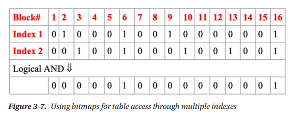
Bitmaps

Used internally by PostgreSQL to facilitate access to other data structures containing data blocks.
A bit is used to indicate if a block contains relevant data.
Multiple indexes can generate bitmaps and be evaluated together.
A bitmap signals to the engine which block may contain records that satisfy both index conditions, but does not guarantee that any single row in that block matches both conditions. This helps to limit number of blocks accessed.
To speed up bitmaps, PostgreSQL builds hierarchical structure for bitmaps to avoid accessing irrelevant portions of the map.

![[image-postgresql-bitmaps.png]]

Other kinds of indexes

Hash Indexes

Use hashing to calculate address of an index block containing an index key.
Much faster than B-Tree, for equality search.
Useless for range search.

R-Tree Indexes

Like a B-Tree, but for spatial data.
Index key represents a rectangle in multi-dimensional space.
Search to return all objects that intersects with query rectangle.

There are many other indexes, e.g. for full text search, or large tables, that are out-of-scope here.

Combining Relations

A set of identical algorithms can be used to support multiple operations like Cartesian product, joins, union, intersection, and even grouping.

Nested Loops

To find product of two tables R and S.
Loop, for each row in R, iterate each row in S, apply filter conditions (if we are evaluating JOIN).
Theoretically, performance cost is proportional to the size of R and S and we can hardly do better.
JOIN operation is the same as applying a product, followed by a filter. Cost remains the same, since all records will be iterated.
Nested loops can be combined with data access algorithms and techniques to create variations, that may improve performance in specific cases. Some e.g.
- using index scans before nested loops.
- loading multiple blocks of R in memory to consolidate and perform a single pass over S.

Hash-based Algorithms

Natural joins (means condition of R join S is equality).
If attributes are equal, the hash of those attributes will also be equal.
Hash-join algorithm has two phase:
- build phase, all tuples of R are stored in buckets according to their hashed value.
- probe phase, all rows in S are sent to matching bucket, and matched with rows from R to produce output.
- these are shown as two physical steps in execution plans.
PostgreSQL uses a more efficient matching algorithm based on Bloom filtering.
Cost is approximately:
- size(R) +
- size(S) +
- (size(R) + size(S))/(number of different values of join attribute)
This performs better than simple nested loops for large tables and large number of different values of join attribute.
If buckets produced in build phase cannot fit into main memory, will need to use hybrid hash join algorithm, that only loads a partition of the tables into main memory, and processing takes place by partition.

Sort-Merge Algorithm

Sort-Merge for natural joins works in two phase:
- Sort phase sorts both tables by the join attributes in ascending order.
- Merge phase scans both tables once, for matching join attribute generate Cartesian product of rows.
Cost is approximately:
- Sort cost =
  - size(R) * log size(R) +
  - size(S) * log size(S)
- Merge cost = same as hash join, but without the cost of build phase.
This algorithm is especially efficient if inputs are already sorted, e.g. in a series of join of the same join attribute.

Comparing Join Algorithms

Depends on use case and situations.
Nested loop is more universal, good for small index-based joins.
Sort-Merge and hash joins are good for larger tables.

Understanding Execution Plans

Use the EXPLAIN command to generate an execution plan from an SQL query.
For the query planner, choosing execution plan is a nondeterministic process.
Even when the plans are identical, execution times may vary with differences in hardware and configuration.

Reading Execution Plans

![[image-postgresql-execution-plan.png]]

Each row contains:
- An operation that will be performed
- Estimated cost, which is accumulated from all previous operations before this current operation. There are two values in the cost:
  - cost to get the first row
  - cost to get all results
- Estimated number of rows of output (based on database statistics)
- Expected average width of a row
These are estimates, and errors grow as more operations are applied.
pgAdmin provides graphical tool to display the plan as a tree.
Operation at the rightmost offset will be executed first.
- Independent leaf nodes can be executed in parallel.
- There is no need to store intermediate results between operations. A row will be pushed to the next operation once generated.
Execution starts from leaf nodes and ends at the root.

How was the plan optimised

Recap, during optimisation, the optimiser will:

Determine the possible orders of operations
Determine the possible execution algorithms for each operation
Compare the costs of different plans
Select the optimal execution plan

Therefore, plans of the same SQL query may vary in:

Order of operations
Algorithms used for joins and other operations (e.g., nested loops, hash join)
Data retrieval methods (e.g., indexes usage, full scan)

The optimiser does not search through all plans in the search space. It relies on optimality principle:

Start with the smallest sub-plan and find the optimal.
Move up the plan tree to search for optimal sub-plan, with descendent nodes already optimised.
Heuristics also helps to reduce search space.

How are costs calculated

The cost of each execution plan depends on:

Cost formulas of algorithms used in the plan
Statistical data on tables and indexes, including distribution of values (this affects selectivity)
System settings (parameters and preferences), such as join_collapse_limit or cpu_index_tuple_cost

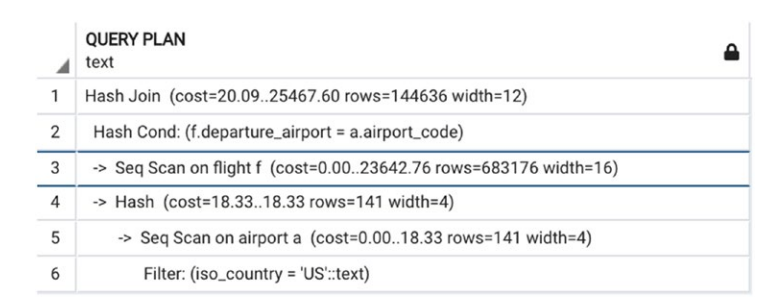
There is no best plan, since the factors affecting cost will change according to database usage. Example from the book:

SELECT flight_id, scheduled_departure
FROM flight f
         JOIN airport a
              ON departure_airport = airport_code
                  AND iso_country = 'US';

Because selectivity of this filter condition iso_country = 'US' is high, the optimised plan will use a full scan.
However, if we change this to a low selectivity condition like iso_country = 'CZ', then the optimised plan will use a bitmap heap scan instead.

Optimisers are not perfect

The optimisers estimate cost using formulas that assumes uniform distribution of data, which only provides an imperfect approximation of real use cases.
The optimisers use database statistics which are accurate for stored tables, but has limited effectiveness on intermediate results of an execution.
The optimisers may miss the optimal plan in their search, because of heuristics, or because query is too complex.

In all these cases, human intervention might be required to fix the situation.

Short Queries and Indexes

A query is short when the number of rows needed to compute its output is small, no matter how large the involved tables are.

Not just the initial input rows need to be small, the intermediate results between operations should also be small.
Short queries may read every row from small tables but read only a small percentage of rows from large tables.
The definition of “small percentage” depends on system parameters, application specifics, actual table sizes, and possibly other factors.

The optimisation goal of short query is therefore to reduce the size of the result set as early as possible. If the most restrictive selection criterion is applied in the first steps of query execution, further sorting, grouping, and even joins will be less expensive. To achieve this, we need indexes.

Details about Indexes

Index Selectivity

The lower the index selectivity, the better the performance for short queries. (e.g. it doesn’t make sense to create an index on population data using gender as the index key, because the selectivity is very high)
We should ensure that search criteria of a query will use indexes.
Among all search criteria, having the most restrictive (the lowest selectivity) criteria satisfied by an index will produce the best performance.
UNIQUE index = for each indexed value, there is only one matching row in the table. Unique indexes has the best selectivity performance.
- PRIMARY KEY is simply a short-hand for UNIQUE and NOT NULL constraints. Primary keys can be composite attributes.
- UNIQUE constraint is nullable.
- the unique index can be created separately from the table instead of being defined as a constraint. However, upon creation all rows in the table will be validated. Index will not be created if validation fails. After creation, subsequent insert/update to the table will be constrained.
FOREIGN KEY is a referential integrity constraint, which does not create an index by default.
- joining and searching foreign key relations will still be slow unless indexes are explicitly created.
Best Practice: Creating index on foreign key column/join column, will not always improve performance. We should only create index is number of distinct values is large enough (low selectivity).

Column Transformation

A column transformation occurs when the search criteria are on some modifications of the values in a column. E.g. casting string value to timestamp type before filtering.
The index on original column attribute cannot be used for search that requires transformation.
A functional index may be required to serve the use case
- create index by applying a function to a column attribute, and storing the transformed value as index key.
Column transformation may be subtle in your search, so your execution plan may be running full sequential scan, when you assume that an index is used.
Some queries may be re-written to produce the same results without transformation, which is one option to optimising.
E.g. when searching for all records created today,
- instead of casting the created_at timestamp column to date type
- to perform an equality comparison to today’s date,
- we can decompose the search condition into a range search on the existing created_at timestamp column,
- range between timestamp at the start of today and timestamp at the end of today.

LIKE Operator

LIKE search criteria is not supported by B-tree, so a full scan will likely be executed.
LIKE search can be re-written as a range search:
- e.g. WHERE last_name like 'johns%' can be decomposed to a range
- WHERE last_name >= 'johns' AND last_name >= 'johnt'
Best Practice: create a pattern search index to support such use cases.
- e.g. text_pattern_ops, varchar_pattern_ops, and bpchar_pattern_ops
- e.g. creation CREATE INDEX test_index ON test_table (col varchar_pattern_ops);
- comparison of text values depends on the locale, which determines character ordering, formatting, which varies by languages/countries.
- use SHOW LC_COLLATE; to see the locale setting in the database.
- LIKE operator on an attribute column with pattern search index will automatically use the index to optimise execution.

Using Multiple Indexes

PostgreSQL will create in-memory bitmaps of multiple indexes to reduce the blocks that will be accessed.

Compound Indexes

Indexes built from multiple columns.
In general, an index on (X,Y,Z) will be used for:
- searches on X,
- searches on XY,
- searches on XYZ,
- and even searches on XZ
- But index on (X,Y,Z) will never be used on searches on Y alone or on YZ.
Best Practice: When creating compound indexes, deciding the columns to include, and the sequence of columns are equally important, and should consider the use cases.
Compound indexes may perform better than using multiple individual indexes when:
- the compound index significantly lower selectivity. (uniqueness only surface from a combination of columns..
- the compound index contains sufficient columns to satisfy the SELECT query (index-only scan is sufficient without table access).

Covering Indexes

Introduced in PostgreSQL 11.
A covering index is specifically designed to include the columns needed by a particular type of query that you run frequently.

CREATE INDEX test_index
    ON test_table
        (X, Y, Z) INCLUDE (W);

The column W is included in the covering index to avoid accessing the table, but it is not used as search criteria.
For small columns, it may not matter if the extra column is indexed for search.
However, for wider columns, the use of covering index helps keep the index key compact.

Excessive Selection Criteria

This refers to the practice of providing additional, redundant filters to prompt the database engine to use specific indexes or reduce the size of join arguments.
Some SQL queries simply cannot be optimised if the search conditions depends on result values from multiple tables.
- Analysing business requirements may reveal that it is not necessary to search through the entire space from data since the dawn of time.
- Excessive selection criteria may be applied to limit the search space of large tables, which the query optimiser can use to re-order queries and optimise execution.

Partial Indexes

Refers to indexes built from only a subset of rows in a table.
- e.g. flights scheduled do not have actual_departure, until the flight takes place.
- create a partial index for only flights with a non-null actual_departure value will help improve search for flights that already took place.
Another use case: searching for retail orders with status = ‘REJECTED’ will automatically use this partial index to narrow search space.

-- possible status values are NEW, ACCEPTED, REJECTED, CANCELLED
CREATE INDEX retail_order_rejected
ON retail_order (id) WHERE status='REJECTED';

Indexes and Join Order

Applying most restrictive selection criteria first with indexes helps reduce intermediate result size.
Intermediate result size can also be minimised by performing semi-joins where one side of the argument significantly capped the size of join results.
Most of the time query planner is able to choose the most optimal plan, unless it was forced by SQL query to select a bad ordering.

Manipulating Index Usage

Avoiding Index Usage

We want to avoid using indexes when:
- A small table is completely read into main memory.
- We need a large proportion of the rows of a table to execute a query.
Most of the time query planner is smart enough to detect that indexes should not be used if it yields poorer performance.
To manually force this, we can apply inconsequential column transformation (e.g. adding zero to numeric values).

Forcing Index Usage

If the query planner is not using your index, it is likely because using the index will yield poorer performance. (PostgreSQL optimizer is smart.)
Best Practice: Let PostgreSQL do its job.

How to Build the Right Indexes

(Traditional) reasons against building too many indexes:
- take up extra space in database.
- slows down insert/update rows with overhead. (Prevailing guidance is to drop indexes before bulk loading, then create them again.)
Times have changed:
- disk storage is cheaper and faster. Fast response is more critical than saving space.
- even if total size of indexes exceeds table size for OLTP systems, it is acceptable.
Best Practices:
- create partial indexes whenever it makes sense. These reduces search space, allows working data to fit in main memory.
- create covering indexes whenever it makes sense. These reduces round trips to the table.
- keep an eye on all indexes, to detect slowness for inserts/updates. Poor performance are usually caused by:
  - unique/primary keys.
  - foreign key references to unique/primary keys in other tables.
  - SQL triggers on inserts/updates.
- pg_stat_all_indexes shows index usage. We can consider removing unused indexes.

Maintaining Indexes for Scalability

As data size grows, index performance may worsen due to:
- index becoming too large to fit into main memory.
- index gets pushed out by indexes for competing queries.
When we design queries and indexes, we aim for them to scale well to a reasonable extent.
- No optimised set up lasts forever.
- keep an eye on data volume growth.
- keep an eye on data distribution.

Long Queries

A query is long if:

selectivity is high for at least one of the large tables. That is, almost all rows contribute to the output (aggregation), even when the output size is small.
or, anything that is not a short query is a long query (LOL)

Overall strategy to optimise long queries is to:

Avoid multiple table scans.
Reduce the size of the result at the earliest possible stage.

Scans and Joins

Full Scans

Full scans are more desirable for long queries.
Index will use more I/O access than full scan due to high selectivity so should be avoided.
However, actual measure of whether full scan is required is decided by PostgreSQL, and is also dependent on hardware specs.

Hash Joins

Hash joins are always more preferable to nested loops as the cost is lower (refer to formula in earlier sections)

Rule of thumb

Index access works well with nested loop.
Sequential scan works well with hash join.
We should look for these indicators to see that query plans meet expectation (our job is to verify the plans).
We should remember to always let PostgreSQL optimizer do its planning job.

Order of Joins

We should always perform most restrictive joins first, even for large tables.

Semi Joins

These are joins that satisfy two conditions:
- Only columns from the first table appear in the result set.
- Rows from first table are not duplicated even when there is more than one match in the second table (removes duplicate).
Queries may not be using the JOIN keyword, but the plan will indicate a semi join.
- e.g. selecting from a table using a column selected from another table. (using EXISTS or IN keywords)
- only EXISTS keyword guarantee a semi join plan.
The optimiser may also choose a regular join, depending on database statistics.
Semi joins by definition cannot increase the size of result set, and is often the most restrictive join in the plan.
Depending on filter conditions of query, semi joins may be most restrictive for large range, but index access may become more restrictive at small ranges.

Anti-Join

A join that returns all rows from first table with no match in second table.
Uses operators NOT EXISTS or NOT IN to define queries.
- only NOT EXISTS guarantees an anti-join
- using OUTER JOIN followed by a filter NULL may also lead to optimiser re-writing the operation as an anti-join.

Manually Specified Join Order

The manual join order of the query will only be respected when we hit the limit set by server param join_collapse_limit (default value is 8).
Within this limit, the optimiser will still create candidate plans and select the best option. Beyond that, the planner will use the specified order.
The higher the join_collapse_limit the longer it will take for planner to choose a plan.
Therefore, setting this param to 1 will always force the join order.
- Another way to force the order is to use common table expressions (CTE).

Grouping

Filter First, Group Last

A common mistake is to figure out how to perform a grouping calculation (on the entire dataset), creating an inline view, then trying to filter for the data required.
This forces suboptimal execution sequence.
Ideally we should allow the data to be filtered as soon as possible as part of the innermost query, if any.

Group First, Select Last

Sometimes, it may be more optimal to perform grouping first, if it reduces the size of intermediate results (before joins).
The inline view can then be used for further grouping in the query.
I think we need to compare query plans to evaluate if it is worthwhile to rewrite the query for such optimization (it may not be obvious to detect this)

Reducing Size/Computation

SET Operation

Using SET operation may prompt the optimiser to select alternate algorithms and may end up with more optimal plans. E.g.
- using EXCEPT instead of NOT EXISTS or NOT IN
- using INTERSECT instead of EXISTS or IN
- using UNION instead of complex selection criteria with OR
On top of the potential performance improvement (not guaranteed), it also improves readability of code.
Note that when using hash joins or SET operations, execution time increase significantly if any datasets cannot fit into the main memory.

Avoiding Multiple Scans

Multiple scans is usually a result of poor schema design. We can only try to write better queries to salvage the imperfect design (if it is beyond our control)
A common design pattern is to use Entity-Attribute-Value (EAV) to store arbitrary attributes for data that is added to serve new use cases only after a system is live in production. (The design is similar to DynamoDB table with entity-relations modelled in a single table).

e.g. Other Table

other_table_user_id	other_table_user_name
0001	John
0002	Mary
0003	William

*e.g. EAV**

eav_user_id	eav_attribute_name	eav_attribute_value
0001	School	Engineering
0002	School	Arts
0003	School	Law
0001	Year	4
0002	Year	5
0003	Year	2

A query that wants to select the school and the year of each student may join the EAV table with the other table twice, generating two full scans.
A way to optimise is to ensure that we join the table only once. Use CASE statements to SELECT the correct values into the view columns.

SELECT user_id,
max(
	CASE WHEN eav_attribute_name = 'School' THEN eav_attribute_value
	ELSE NULL END
) as school,
max(
	CASE WHEN eav_attribute_name = 'Year' THEN eav_attribute_value
	ELSE NULL END
) as year
...
GROUP BY user_id;

Aggregation functions like max can help to eliminate empty rows from joining the EAV only once.
As additional optimisation (if applicable), we may filter/group values in the EAV before joining (please refer to the techniques mentioned above).

Additional Techniques

Temporary Tables

Created using the command CREATE TEMP TABLE table_name AS SELECT ....
Will be dropped when session disconnects.
Potential problems:
- Abused by developers who write each intermediate steps of computation to a temp table.
  - Subsequent queries will not be able to use indexes from original source table. (Will need to build need indexes).
  - Blocks query rewrites as optimizer do not have control over the entire query (it is forced to break the execution to persist intermediate results in temp tables).
- New temp tables do not have statistics to assist the optimizer.
- Temp tables competes for storage resource used by certain operations like joins and groupings.
- Excessive I/O as temp tables are written to disk.

Common Table Expression (CTE)

Can be thought of as temp table for a single query.
Each auxiliary statement (the CTE) in a WITH clause can be attached to a primary statement.
Before PostgreSQL 12, CTEs are executed as temp table, materialised in main memory with disk failover. Therefore, there is no performance improvements over temp tables.
The purpose of CTEs are to allow reuse of a same sub-query more than once in a statement.
- This creates an optimisation fence, where CTEs will be planned separately by the optimiser.
From PostgreSQL 12 onwards, if CTE is used only once in a SELECT statement with no recursion, the optimisation fence will be removed. The CTE will be rewritten and inlined as part of the outer query.
- This new feature can be ignored using the MATERIALIZED keyword. eg. WITH cte AS MATERIALIZED ....
Therefore, CTEs can be used to improve readability, as long as it does not create unintended temp tables.

Views

A view is a database object that stores a query that defines a virtual table.
When selecting on top of a view, the original query stored in the view will be inlined as sub-queries by the optimiser.
Potential problems of views:
- May result in sub-optimal execution if the optimiser is unable to rewrite the statement, and the use of the view accidentally forced a sub-optimal execution.
- The view abstracts the details of the underlying database objects (good for usability but…)
- It may be used by developers to make inefficient queries without knowing the details. E.g. querying without the help of indexes on a view, when the required indexes do exist on the underlying tables.
- PostgreSQL internally creates rules, triggers, and automatic updates to make views behave like tables, making it an extremely sophisticated object.
Views do not provide any performance benefits!
The best use case for views would be to act as a security layer, or to define a selection properly for reporting purposes.

Materialized Views

A materialised view is a database object that combines both a query definition and a table to store the results of the query at the time it is run.
Subsequent reading of the view will show stale data (from the table).
There is no way to update the data, besides using REFRESH command to run the predefined query in the view.
- Based on current PostgreSQL implementation, during a refresh, the table will be truncated, and all data reinserted.
- On error, the refresh will roll back to the last version.
- If refreshed with the CONCURRENTLY keyword, the view will not be locked (available for read during refresh). But the view must have a unique index.
Indexes can be created on materialised views.
Materialised views cannot have primary/foreign keys.
Material views may be good for the following use cases:
- data that seldom changes
- it is not critical to have live data
- it will be used by many different queries, and many reads between refreshes.

Dependencies

Creating a view/materialised view creates a dependency on the underlying tables (or underlying materialised views).
ALTER or DROP on the underlying database objects are not permitted unless using CASCADE.
Even a simple modification on an underlying table, e.g. adding a column, that does not affect the views, will require the view to be dropped and rebuilt.
This is the unfortunate limitation of PostgreSQL.
If a web of dependencies has been created, altering a table may be extremely slow.

Partitioning

Partitioning is relatively new to PostgreSQL, starting from version 10.
Range partitioning = all rows in a partition has attribute values within a certain range.
Adding/Dropping a partition can be significantly faster than working on a single table with massive data.
Partitioning may improve query performance.
- Partitions may be distributed across different servers.
- Certain scans may only need to access a single partition.
- Indexes may also be built on the partition (within the partition), but will only benefit if query do not require multiple partition access.

Parallelism

Parallel execution is relatively new to PostgreSQL, starting from version 10.
Good for massive scans and hash joins where the work can be split up into multiple unit.
Sometimes, optimiser may replace sequential execution (index-based) with parallel table scan, due to imprecise database statistics, which may perform worse than sequential execution.
Use server settings to ensure that optimiser will consider parallel algorithms, and let the optimiser do its job.
Parallel execution is often view as a silver bullet, but it cannot fix poor design.

Optimise Data Modification

Usually consists of optimising two parts
- Optimising the selection of data to be updated (use strategy described above)
- Optimising the data update itself (use strategy in this new section)

Understanding Data Modification Concepts

Low-Level Input/Output

Read operations requires all required database blocks to be fetched from disk to main memory to complete.
Write operations however, do not require actual modified database blocks to be written to disk to complete.
- This can happen in the background. Operation is deemed complete once changes are registered in main memory.
- So it will appear fast to users, but it still takes up system resources.
- Heavy load of data modification operations will also slow down incoming modification operations due to concurrency control.

Concurrency Control

Lock waiting (transactions trying to update the same data) can slow down operations.
Flushing Write-Ahead Logs (WAL) too frequently leads to disk I/O, slows down performance.
- This happens when we do not use transaction control (by default every DML will be one transaction and gets committed immediately, therefore WAL gets flushed)
For PostgreSQL, new updated row/deleted row are not overwritten.
- They are stored as dead row while a new row take its place.
- Dead rows are cleaned out by VACUUM operation.
PostgreSQL uses Multi-version Concurrency Control (MVCC), Snapshot Isolation (SI) model.
- Transactions always read latest committed rows.
- Concurrent write to same row is not allowed and only one transaction will hold the lock.
- Lock is released if transaction aborts.
- If transaction commits, then behavior depends on the configured isolation level in the transaction.
  - READ COMMITTED is the default, waiting transaction will read the new committed data and proceed.
  - REPEATABLE READ, the waiting transaction will be aborted since initially read data differs from current data.
  - There are other levels not covered.

Data Modification and Indexes

Rule of thumb, one extra index increase data update/delete time by approximately 1%.
CREATE INDEX locks the entire while CREATE INDEX CONCURRENTLY does not, but takes longer.
PostgreSQL uses the Heap-Only Tuples (HOT) technique to reduce index updates when new row is inserted.
- if the same block has sufficient free space for new row data and
- no index columns need modification
- then no indexes will be modified.

Mass Updates

if massive updates create a lot of dead rows, that means blocks are not used efficiently.
operations will read a lot of blocks, incurring disk I/O.
however, PostgreSQL auto-vacuuming should still be good enough. Engineers simply need to tune the configurations appropriately.

Frequent Updates

very frequent updates also results in dead rows and therefore inefficient block usage.
if auto-vacuum cannot keep up with the frequency, we can also tune the fillfactor storage parameter.
- low fillfactor means a new block will only utilise a small amount of space.
- the free space will be reserved for update operations.
- since the block has free space to store new versioned rows, indexes do not need to be updated.
- however, the tradeoff is operations will need to fetch many blocks inefficiently (when updates didn’t happen).

Referential Integrity and Triggers

Foreign key constraints will slow down inserts (on child table) due to additional checks.
Foreign key constraints will also slow down updates and deletes (on parent table).
Constraint checks are implemented internally as system triggers.
Therefore, triggers also slow down performance.
However, it also depends on situation and size of data.
This also does not mean we should avoid constraints and triggers (they are important and valuable).

Design

Alternatives to RDBMS

It is hard to replace RDBMS because fundamentally the query language (SQL) is based on boolean logic and does not specify the way to store data. Eventually all other types of databases chose to support SQL as one of their query language option.

Entity-Attribute-Value (EAV)

Covered in earlier section, the EAV contains 3 columns (entity id, attribute id, value).
It is popular and offers flexibility when requirements are unclear.
Performance is still slow compare to traditional relational models.
Cannot easily enforce referential integrity, or data validation constraints.

Key-Value Model

A single primary key, with other attributes stored as a complex object. (like DynamoDB).
Limits the database engine from performing more complex operations on other attributes, without retrieving the full object.
PostgreSQL new JSONB support provides a similar experience.
Again like EAV it is hard to enforce referential integrity, or data validation constraints.

Hierarchical Model

Typical document stores. (like MongoDB).
Popular because it is intuitive to understand.
Works great when data can be modelled in a single hierarchy.
Gets more complex when data fits multiple hierarchy.

Combining the best of all worlds

PostgreSQL provides features (such as JSONB support) that allows us to gain the benefit of all the above databases without using different technologies.
PostgreSQL also provide Foreign Data Wrappers (FDW) to abstract the access to other databases (DBMS and more) transparently.

Flexibility vs Efficiency & Correctness tradeoff

Storing values as text, regardless of type, will sacrifice correctness.
It will also be difficult to perform type-specific comparisons (e.g. date comparison) when data are stored as text.
- And as a result, indexes will also not work so well for inequality searches.
JSONB best serves use cases that requires the retrieval of the entire object, instead of attributes within objects.

Normalisation

Normalisation is typically misunderstood and used/not used properly.
In a nutshell, it is used to decompose data into multiple tables, depending only on the same primary key, to reduce repetition.
Usually if Entity-Relation (ER) models are designed properly, the schemas are naturally normalized.
But the importance of normalisation again depends on situation.
- The primary purpose should not be performance optimisation.
- Normalisation provides cleaner structure, supports referential integrity constraints.
Ideally, a clean logical structure should be provided for the application based on a storage structure optimized for performance.

Surrogate Keys

Unique values generated to identify objects. (In PostgreSQL they are values selected from sequence).
Defining a column as serial type naturally obtains the next generated value when a row is inserted.
It is not necessary to have a blanket policy to create surrogate keys on every table.
- It is detrimental if the key has no bearing to real world relations.
- It is even worst if the table also stores a unique identifier from the real world relations.
In some cases, it is useful to have an internal identifier, when the table have data with the following characteristics:
- the real world identifier gets repeated after a short period of time and therefore is not unique.
- data defined by multiple source systems with different external identifier conventions.
- in the future, the data may lose their identifier or update their identifier due to system changes.
- data needs to be joined with other tables that may be extremely large using existing identifiers, and may be optimized by surrogate keys.

App Development and Performance

This section focuses on optimising processes instead of queries. This aspect is often neglected but can bring about huge impact.

Response time is a huge non-functional requirement for all systems, regardless of industry and use cases.
Application and Database can both be working perfectly (in terms of their own metrics)
and yet, the interactions between the two systems slows down overall response time for the end user (which is the more important metric from the user’s perspective)

Impedance Mismatch

The power of the expressiveness and efficiency of database query languages (declarative) does not match the strengths of imperative programming languages.
Even though both can have great strength, they might deliver less power than expected.

Interface between Application and Database

JDBC and ODBC are generic interfaces that simply cannot offer the full power of the database to the application.
ORMs are worse.
- They abstract all details from the application.
- ORMs often end up with N+1 queries because as a generic tool it cannot satisfy all use cases.
Trying to abstract storage/persistence implementation details from the business logic in a layered approached often results in some sacrifice.
- objects have no knowledge of each other, resulting in inefficient query (kind of like N+1 queries problem) at the service layer to bring different objects together.

A Better Approach

The above can be summarised as two closely related problems:

Inability to transfer all the data at once to the application (to think and operate in sets).
Inability to transfer complex objects without disassembling them before the data transfer to/from the application.

In theory PostgreSQL should be able solve the above by using a single query to return a set because:

it is an object-relational database (JSONB support)
it allows the creation of custom types
it has functions that can return sets, including sets of records

Functions

User-Defined Function

Besides internal functions, we can create custom functions using:
- SQL
- C
- Procedural Language (PL), which includes by default:
  - PL/pgSQL
  - PL/Tcl
  - PL/Perl
  - PL/Python
The database engine only captures the following metadata about the function:
- name
- list of params
- return type
- language of the function code
The function body itself is stored as string literal, and will be passed to language-specific special handlers to parse/execute at runtime.
PostgreSQL didn’t support stored procedures in the past. Some outdated guide may recommend packaging multiple statements together using a function that returns void to emulate a stored procedure.
PostgreSQL supports function overloading (polymorphic behavior).
Supports exception handling using EXCEPTION and WHEN keywords. This prevents query from failing in a SELECT statement if the function can return a fallback value when it cannot process the input.
Function can also work with DML to insert/update/delete data.
Please refer to official documentation for full function definition syntax.

Function Execution Internals (PostgreSQL)

Functions are not compiled. The source code will be stored. Therefore, PostgreSQL is unable to detect syntax errors like wrong column name.
Function code will be interpreted when called.
- an instruction tree will be produced the first time function is called within a session.
- only when the execution path reaches any specific commands in this function’s instruction trees, then an actual SQL statement will be prepared.
- in other words, if the function contains conditional logic, and one of the conditional branches has syntax error, it may take a long time to detect if that branch was never executed.
Transactions cannot be initiated inside a function.
Functions also do not generate execution plan, so the optimiser will not know the cost of a function (unless the function was defined using COST keyword and the engineer manually supplied an arbitrary value. This is quite dangerous if you do not know what you are doing).

Functions Performance

Performance can be bad because to the optimiser, the function is a blackbox with no database statistics to help improve the plan.
The function code may introduce inefficiencies to a query.
Perhaps the best use of function is not to improve a single query performance, but to improve overall process.

User Defined Types

Can be DOMAIN, ENUM, RANGE
Can even be a composite type which represents a record
- the definition consists of attribute names and data type of each attribute
Functions can return sets of composite types.
Composite types can contain elements which are defined as other composite types.
- this allows us to represent complex nested objects in our results.
- unfortunately, the details about the structure (nested attribute names and data types) will not be revealed in the result, which limits the use of this approach as a solution to nested object.
Functions that depends on user defined types must first be dropped and later recreated, if the types need to be modified.

Function Security

Supplying the SECURITY parameter will change the access control behaviour of the function.
SECURITY INVOKER is the default. Function will run with permissions of the user calling it. User must have access to underlying database objects used in the function.
SECURITY DEFINER will use the function creator’s permission instead, even if the function caller has no permission.
access to all functions are granted to PUBLIC by default (so everyone can be a function user).

Business Logic

When deciding what can go to the database and what has to stay in the application, a decisive factor is whether bringing the dependencies into the database would improve performance (facilitate joins or enable the use of indexes).
If so, the logic is moved into a function and considered “database logic”; otherwise, data is returned to the application for further processing of business logic.

Functions in OLAP

Can be used to parameterise a view (by selecting records using functions)
Provides an abstraction from underlying view/table

Stored Procedures

They are like functions that do not return any values.
They also allow transactions to commit and rollback within the procedure body (functions do not allow this)

Exception Handling

Exceptions can be handled by separate inner blocks of the function

Dynamic SQL

Generating SQL code dynamically, to be executed by the database engine.
Advantage specific to Postgres:
- Postgres optimise execution for specific values, and at the last step of planning.
- Using dynamic SQL ensures that your queries are always optimised.
General approach is to generate dynamic SQL code (in text) within a function, and run it.
- It is able to provide consistent performance, because the optimisation do not depend on database session cache.
- If we save the SQL code as a function instead, performance will be affected by session cache, and the cache may currently contain a sub-optimal plan.
- However, dynamic SQL is harder to debug and develop.
No worries about SQL injection, if input params from users are sanitised, and SQL code are generated from database functions (not from users directly).

Flexibles JOINS

Since SQL code are constructed on the fly, certain JOINS can be omitted depending on input params.
It can also force the optimiser to execute index joins over hash joins.
This provides significant performance improvement.

Avoiding ORMs

This is a golden quote from the book:

Often, new development methodologies require application developers to make significant changes to the development process, which inevitably leads to lower productivity. It is not unusual for potential performance gains to fail to justify the increase in development time. After all, developer time is the most expensive resource in any project.

This is applicable to the entire software engineering industry in general.
It is often not worth the effort to migrate to the next new, shiny, and trendy things on a whim, derailing the entire product development roadmap.

NORM as an alternative

An example framework is provided by the authors on GitHub
Contract driven approach to develop the interface between database models and application models.
ORM are generic tools, and therefore always causes N+1 query problem.
Having customised and specific database functions to return result sets that can be serialized, and then deserialized by the application to JSON objects.
- Can be optimised to run only one query in the database.
- Combining with dynamic SQL provides a powerful way to run complex queries (with CASE WHEN to selectively JOIN and search for values depending on input params).
- Application development only need to rely on the interface, that promises the return of deserialised JSON objects.
This approach does not store data directly as JSON because it will lead to duplicated data (typical of NoSQL document store).

Complex Filtering and Search

This chapter covers use cases that cannot be efficiently supported by B-trees.

Full Text Search

The search model used by Postgres is a simple Boolean model (internet search engines use more complex models).
A document is a list of terms.
- Words with the same meaning are mapped to the same term, using linguistic tools.
- Linguistic rules are defined in a configuration in Postgres, but is language dependent.
- Trigrams, converting text into a set of 3-character sequences, is a language independent processing.
Result of text processing is of ts_vector type (which is a list of terms).
A query is represented as ts_query type (also a list of terms, with logical AND, OR, NOT connectors).
Logical match will be performed, and the result is Boolean. The ts_vector either match the ts_query or not.
Full text search in Postgres can work without indexes, but can also be optimised with special indexes. Use the @@ command in the WHERE clause to query.

Multidimensional/Spatial Search

Default multi-column indexes has search priority based on the order of columns, which cannot work for multidimensional data that requires all dimensions to be treated symmetrically.
The default also cannot support range queries and nearest-neighbour queries for spatial data.
There are specialised indexes in Postgres for these use cases.

Generalised Index Types

Indexes created by B-tree by default, but we can specify the following specialised types: hash, GIST, spgist, GIN, and BRIN.

GIST Indexes

This is a family of index structures, specialised for different multidimensional data types.
e.g. data can be represented as multidimensional point, and query is a multidimensional rectangle over the space.

Indexes for Full Text Search

GIN (Generalised Inverted) can be used.
- Document has a list of terms after processing (ts_vector)
- This index is created from each term in the list, and map the term to a list of documents containing the same term (hence, inverted)
- A search using this index can quickly find a relevant documents.
- GIN can be a functional index, that either persist the ts_vector of the document or not. If persisted, the search can be done without language specific configurations.
- GIN can also work for arrays of values, multivalued attributes.
GIST can also be used, but data will be indexed as bitmaps.
- Each term in the document will be hashed, and the hash value is represented as a bit in the map.
- A bitmap of a document will indicate existence of all the terms (may have hash conflicts which is fine since it is an approximate result, and Postgres will recheck the ts_vector before returning).
- Query will also be converted to bitmap.
- The search performs a simple logical matching of bitmaps.
- But if documents have a lot of terms, hash conflict will be high, and GIST will become less effective.

BRIN for Very Large Tables

Other databases support clustered indexes (data stored in the same order in the block as the index).
- Clustered indexes are usually sparse indexes (index only need to store the first row in a block, and the block can be scanned)
Sparse index only stores a fraction of data of the column, but can still work effectively.
Dense indexes need to store all data in the column it has indexed.
Postgres do not support clustered indexes because it does not allow users to control how data is ordered in the block.
- However, if the data in the tables are append-only, and always appended in order.
- And if we are interested in indexing their appended order e.g. the timestamp.
- We can use BRIN (Block Range Index)
BRIN works similar to how the typical clustered index works as described above.
- However, it becomes ineffective if data appears in multiple blocks and gets appended out of the order.
- BRIN index a summary of the columns within a block range.
- The summary can be e.g. the min-max value of timestamp of rows within the block, or a multidimensional rectangle bounding the records of spatial data.
- Summarisation is expensive, so we can configure it to run on trigger (for small load), delay it to run with vacuum, or run it manually.

Indexing JSON and JSONB

JSON type is stored as string, while JSONB is stored as binary.
JSONB allows more performant indexes to be built and can satisfy more complex search use cases.
Special indexes mentioned above can be built to search JSONB. However,
- Performance will still not be as good as the usual B-tree indexes.
- Certain indexes like GIN do not support certain attribute values (like datetime) or complex searches. You may need to further enhance the data by persisting search terms alongside the record to specially facilitate full text search.
- Data in JSONB are denormalized and duplicated and may be out of date especially for foreign key relations, and will need to be refreshed periodically (perhaps through triggers).

The Ultimate Optimization Algorithm

![[image-postgresql-decision-steps.png]]

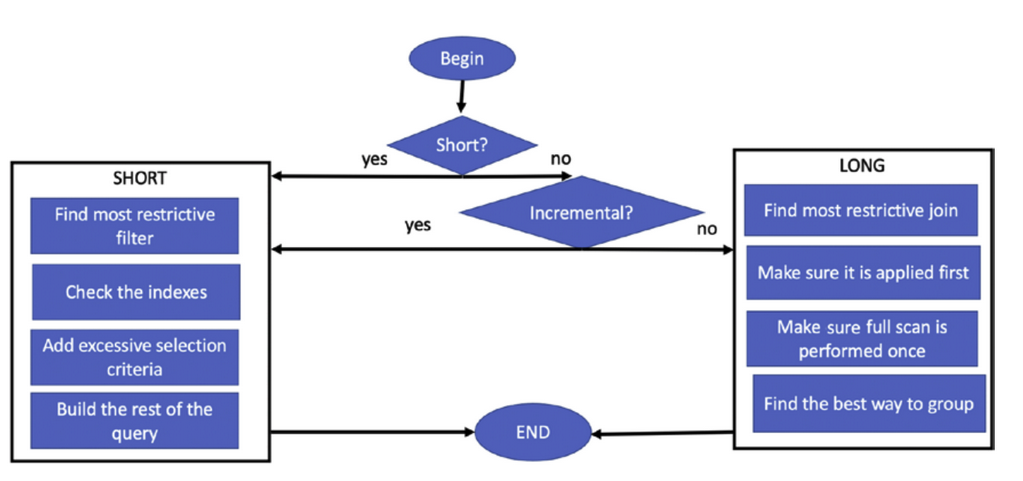
Other Tips

introduce joins one table at a time
observe the execution plan to verify if execution is ideal

Other Considerations

For parameterised queries, different parameter values may change the most restrictive criteria of the query
Dynamic SQL may also change the most restrictive criteria
Functions may degrade performance but it is needed for dynamic SQL
Changing database design instead of optimising the queries, if applicable, is also a good solution

Share on

X Facebook LinkedIn Bluesky